10 Minute Mental Model: Little's law, the giant governing Throughput & Latency
Learn more about the 10 Minute Mental Model series
Canonical Example
I am going to write a GPU program using CUDA. I think it will be fast but I am not sure if it can be significantly faster. Am I getting the most out of the hardware? Do I need to write the program, then measure and improve performance or can I architect it in sympathy with the hardware and get most of the performance the first go around before any profiling?
If you are familiar with this feeling, be it for GPU, Storage or NIC hardware, this post may help a little (no pun intended) bit!
Understanding Throughput & Latency: A museum example
Imagine a museum where people queue to get in and once they are in, take different routes and spend different amounts of time in the museum before exiting it. What are some metrics to monitor the logistical functioning of the museum? The common ones are:
- Latency: How long does a person stay in the system (either in the queue or in the museum)
- Throughput: How many people exit the museum per minute
-
Reciprocal Throughput: What’s the average spacing (in minutes) between two consecutve people
exiting the museum. This is just
1/Throughputand can be more intuitive in some cases
What’s the relevance of the museum example? In typical software, museum-like systems are everywhere. For example, to read a disk, the request is first queued by the OS and then dispatched (potentially after coalescing with other requests) to disk. The disk then has its own queuing system. It’s not just disk, but pretty much all limited resources follow the same pattern; CPU threads are queued waiting for a chance to run, network packets are queued on both send and receieve and so on. If you want to improve performance of any of these subsytems, you’ll need reliable metrics. Those metrics will be similar to what one might monitor for a museum.
Why museum? Because latency and reciprocal throughput are orders of magnitude apart. In a typical
museum, Latency is order of hours while Reciprocal Throughput is on the order of secs. When
reasoning about programs, it is easy to conflate the two metrics because they are purely abstract
concepts whereas a physical example like a museum makes it difficult to conflate.
Why these two metrics vs others? Because they tie into economics.
- A high throughput museum amortizes their fixed costs over larger number of people
- A low latency museum makes for a better visitor experience
Analogously, in software too, they tie into economics.
- High throughput = we get more work done for the same hardware
- Low latency = fast response for an end user
Little’s Law
All else equal, we want higher throughput and lower latency; so can we keep improving them simultaneously ad nauseam? And if not, why not?
It turns out that Little’s law places some limits.
Little’s Law (wiki)
Average Throughput x Average Latency = Average number of things in the system
| System | Throughput metric | Latency metric | Number of things in the system metric | Comment |
|---|---|---|---|---|
| SSD | IOPS = IO operations per second | Operation latency | Queue Depth = Outstanding IOPs inside the SSD. | On a single core, async IO can maintain a large queue depth so the SSD is always working on as many requests as possible while sync io can only maintain QD=1. |
| CPU (assume Thread per Task) | Tasks per second | Task latency | Number of tasks = number of threads | When your tasks block a lot (for example, file server blocking on file reads) and the tasks are synchronous (no async/reactive programming), CPU utilization will be very low. You need a lot of threads in the system to utilize all the available CPU cycles. Java’s Virtual Threads allows millions of virtual threads (tasks) to coexist at the same time and switches them cheaply when blocked. This keeps CPU cycles utilized without resorting to async or reactive programming. |
| GPU | Warps per second | Warp latency | Number of Warps | Warp = ~32 threads in Single Instruction Multiple Threads mode. You need a lot of blocks (warps are subsets of blocks) to keep the GPUs fed while some warps need to be switched out waiting on memory. Unlike thread switching, warp switching is very fast (a few cycles), so they get switched even when waiting on memory. |
| Memory Buffers when writing to disk | Disk’s write bandwidth: blocks (say block = 4K bytes) per second | Latency of a single block write | Number of bytes (blocks * blockSize) in memory holding data that the disk is currently writing (the so called buffers) |
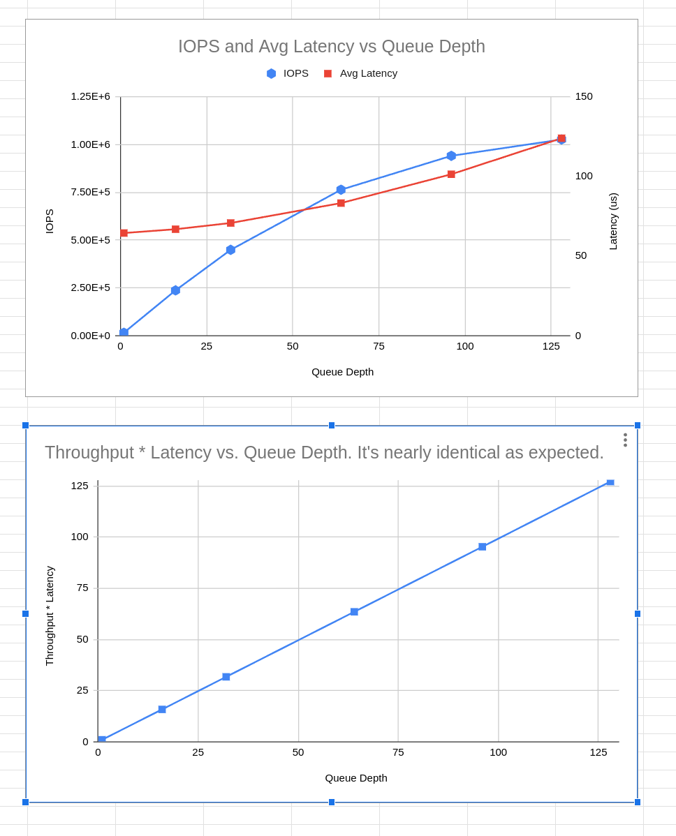
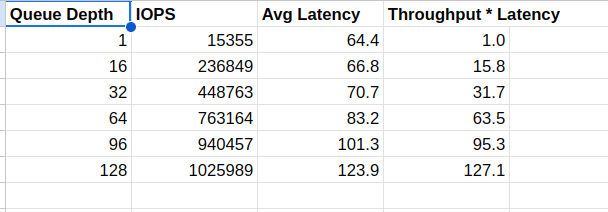
The charts below demonstrate Little’s law in action. These are real numbers from an SSD that is
rated for 1M 4K random read IOPS, tested at various queue depths. That is, the testing mechanism
(fio) ensures that QD requests are outstanding at any moment. Notice how the IOPS linearly
increases with QD while latency remains roughly flat until depth 64. Beyond that, latency
starts climbing noticeably while the disk reaches its saturation point of 1M IOPS. I didn’t capture
the test results for QD 256 in this graph, but compared to QD 128, latency doubles while IOPS
remains the same. This is because QD 128 already saturated the IOPS available on the SSD.


Using Little’s Law in practice
Little’s law helps saturate hardware. Example: If an SSD is capable of 1M IOPS (many today are) at 100 us IOP latency, we know that queue depth should be roughly 100 to saturate the SSD. Going beyond this number will just blow up the latency because requests are just going to be sitting in queue instead of being serviced in parallel by the SSD.
Little’s law informs software design. Example: If we know how much data our batch job has to get through and have a rough requirement of latency, we can estimate the average memory usage. Depending upon whether this number is acceptable or too high, we can play with other design parameters.
Wrapping up
Anywhere there’s a queue, there’s Little’s law lurking. And queues are everywhere in software. Now, different applications will want different tradeoffs. A financial exchange order book management system might care about latency the most (and scaleout to handle volume) while most background pipelines of web companies (say Google’s indexing pipelines) will typically prioritize throughput for economic reasons - you want to get more done with the hardware you have. Any which way, Little’s law helps estimate requirements and refine the design as you juggle design parameters.
Enjoy Reading This Article?
Here are some more articles you might like to read next: